Introduction
This vignette will show you how to run the interaction analyses using
Haplin
package.
Reading data
First, we need to read two datasets: DNA methylation and genotype. We’ll use simulated data here.
library(HaplinMethyl)
#> Loading required package: Haplin

ex_path <- system.file("extdata", package = "HaplinMethyl")
ex_file <- "env_data_test.dat"
ex_out_file <- "dnam_ex"

dnam_ex <- envDataRead(
  file.in = ex_file,
  dir.in = ex_path,
  file.out = ex_out_file,
  sep = " ",
  overwrite = TRUE
)
#> The output file(s) exist!
#> Reading the data in chunks...
#>  -- chunk 1--
#>  -- chunk 2--
#> ... done reading.
#> Preparing data...
#> ... done preparing
#> Saving data...
#> ... saved to file: ./dnam_ex_env.ffData

ex_gen_file <- "sim1"
gen_ex <- genDataLoad(
  filename = ex_gen_file,
  dir.in = ex_path
)
Let’s take a look at it
dnam_ex
#> This is continuous environmental data read in by 'envDataRead'
#> with 400 columns
#> and 200 rows.
showRaw(dnam_ex)
#> opening ff /tmp/RtmpHoavNS/ff/ff52f9d3308edaf.ff
#>           cg1        cg2        cg3       cg4       cg5
#> id1 0.2045598 0.38376996 0.76001042 0.8731273 0.7625753
#> id2 0.2593365 0.41689855 0.94649631 0.9673046 0.4619886
#> id3 0.9912362 0.91398561 0.07621296 0.3841574 0.7026818
#> id4 0.4740415 0.04124038 0.56624919 0.4589275 0.4461102
#> id5 0.7989879 0.52987689 0.66167605 0.1056240 0.3917910
#> attr(,"Csingle")
#> [1] TRUE

gen_ex
#> This is raw genetic data read in through genDataRead.
#>
#> It contains the following parts:
#>    cov.data, gen.data, aux
#>
#> with following dimensions:
#>   - covariate variables =  cov.1
#>       (total  1  covariate variables),
#>   - number of markers =  1 ,
#>   - number of data lines =  200
showGen(gen_ex)
#> Warning in showGen(gen_ex): It appears that your data has less markers (1) than
#> requested (5), adjusting accordingly.
#> opening ff /tmp/RtmpHoavNS/ff/tmp/RtmpekQIls/ff/ff164011e6d830.ff
#> ff (open) byte length=30 (30) dim=c(5,6) dimorder=c(1,2) levels: 1 2
#>      l_m1_a_m l_m1_b_m l_m1_a_f l_m1_b_f l_m1_a_c l_m1_b_c
#> [1,]        1        1        2        1        1        1
#> [2,]        1        1        2        2        2        1
#> [3,]        1        2        1        1        1        2
#> [4,]        1        1        2        2        2        1
#> [5,]        1        2        2        2        2        1
The genotype in the example is coded as 1 and 2 instead of a specific base letter (e.g., A and T, or A and C) and there is only one marker. The order of the columns is as follows: maternal allele 1 (A1), maternal A2, paternal A1, paternal A2, child’s A1, and child’s A2.
Creating the strata
Let’s assume that we know that the first three methylation sites are near the marker that is in the genotype dataset. Thus, we need to extract those methylation sites first.
dnam_ex_subset <- envDataSubset(
  env.data = dnam_ex,
  col.ids = 1:3,
  file.out = "dnam_subset"
)
#> Will select 3 columns.
#> Saving data...
#> ... saved to files: ./dnam_subset_env.ffData, ./dnam_subset_env.RData
dnam_ex_subset
#> This is continuous environmental data read in by 'envDataRead'
#> with 3 columns
#> and 200 rows.
Next, let’s create one variable that gives division of the samples into strata based on the summarized methylation level over the three chosen methylation sites.
dnam_ex_cat <- envDataCategorize(
  env.data = dnam_ex_subset,
  breaks = 3,
  file.out = "dnam_cat"
)
#> opening ff /tmp/RtmpHoavNS/ff/ff52f9d356db393.ff
#> Creating categories: 1,2,3
#> Saving data...
#> ... saved to file: ./dnam_cat_gen.ffData
dnam_ex_cat
#> This is categorical environmental data read in by 'envDataRead'
#> with 1 columns
#> and 200 rows.
showRaw(dnam_ex_cat)
#> opening ff /tmp/RtmpHoavNS/ff/ff52f9d6918ae3d.ff
#>     [,1]
#> id1 2
#> id2 2
#> id3 3
#> id4 1
#> id5 3
#> attr(,"vmode")
#> [1] byte
#> Levels: 1 2 3
Adding the strata variable
Now, the strata variable needs to be added to the genotype dataset.
NB: be careful to check that the order of the samples is the same in the stratified DNA methylation data as in the genotype data!
new_strata <- showRaw(dnam_ex_cat, rows = 1:nrows(dnam_ex_cat))
gen_ex_strat <- addCovar(
  data.in = gen_ex,
  covar = new_strata,
  c.name = "dnam_c"
)
gen_ex_strat
#> This is raw genetic data read in through genDataRead.
#>
#> It contains the following parts:
#>    cov.data, gen.data, aux
#>
#> with following dimensions:
#>   - covariate variables =  cov.1, dnam_c
#>       (total  2  covariate variables),
#>   - number of markers =  1 ,
#>   - number of data lines =  200
showPheno(gen_ex_strat)
#>     cov.1 dnam_c
#> id1 "1"   "2"
#> id2 "1"   "2"
#> id3 "1"   "3"
#> id4 "1"   "1"
#> id5 "1"   "3"
Preparing genotype data
Haplin requires pre-processing of the genotype data before any analysis can be made.
gen_ex_strat_prep <- genDataPreprocess(
  data.in = gen_ex_strat,
  file.out = "gen_strat_prep"
)
#> Reading the marker names...
#> Warning: No map file given, map file empty or the number of map file rows not
#> equal to the number of markers in data; will generate dummy marker names.
#> ...done
#> Recoding covariate data...
#> ...done
#> Recoding genetic data (no. of loci: 1)...
#>    ...running on only one CPU core! This may take some time...
#>    ...checking alleles per SNP...
#>    ...done, all alleles: 1 2
#>    ...recoding SNPs...
#>    ...done
#> Saving data...
#> ... saved to files: ./gen_strat_prep_gen.ffData ,  ./gen_strat_prep_gen.RData
gen_ex_strat_prep
#>
#>      This is preprocessed data, ready for haplin analysis.
#>
#>      It contains the following parts:
#>    cov.data, gen.data, aux
#>
#>      with following dimensions:
#>    - number of covariate variables =  2 ,  - number of markers =  1 ,  - number of individuals/families =  200
Run the analysis
Gene-methylation interactions
Finally, we can run the analysis by using
haplinStrat
g_x_me_results <- haplinStrat(
  data = gen_ex_strat_prep,
  strata = 2
)
#>
#> ## Running haplinStrat ##
#>
#> Selected stratification variable: dnam_c.c
#> Frequency distribution of stratification variable:
#>  1  2  3
#> 67 66 67
#>
#> Running Haplin on full data file...
#> opening ff /tmp/RtmpHoavNS/ff/ff52f9d6e480ef5.ff
#> Done
#>
#> Running Haplin on stratum "1"...Done
#>
#> Running Haplin on stratum "2"...Done
#>
#> Running Haplin on stratum "3"...Done
The resulting object is a list of results, with estimates per stratum and for pooled sample.
names(g_x_me_results)
#> [1] "all" "1"   "2"   "3"
g_x_me_results$all
#> This is the result of a haplin run.
#> Number of data lines used: 200 | Number of haplotypes used: 2
#> Please use the "summary", "plot", "haptable" or "output" functions to obtain
#>  more details.
haptable(g_x_me_results)
#>   stratum row.str marker alleles  counts    HWE.pv Original After.rem.NA
#> 1     all       1     m1     1/2 607/593 0.3708224      200          200
#> 2     all       2   <NA>    <NA>    <NA>        NA      200          200
#> 3       1       1     m1     1/2 178/224 0.4912064       67           67
#> 4       1       2   <NA>    <NA>    <NA>        NA       67           67
#> 5       2       1     m1     1/2 206/190 0.6861466       66           66
#> 6       2       2   <NA>    <NA>    <NA>        NA       66           66
#> 7       3       1     m1     1/2 223/179 0.1415450       67           67
#> 8       3       2   <NA>    <NA>    <NA>        NA       67           67
#>   After.rem.Mend.inc. After.rem.unused.haplos pv.overall haplos haplofreq
#> 1                 200                     200  0.3249067      1 0.5177906
#> 2                 200                     200  0.3249067      2 0.4822094
#> 3                  67                      67  0.4425462      1 0.4919781
#> 4                  67                      67  0.4425462      2 0.5080219
#> 5                  66                      66  0.4570745      1 0.5309276
#> 6                  66                      66  0.4570745      2 0.4690724
#> 7                  67                      67  0.3942638      1 0.5306729
#> 8                  67                      67  0.3942638      2 0.4693271
#>   haplofreq.lower haplofreq.upper reference   RR.est.  RR.lower RR.upper
#> 1       0.4687235       0.5660839       ref 1.0000000 1.0000000 1.000000
#> 2       0.4339161       0.5312765        -  0.8789336 0.5957902 1.300486
#> 3       0.4080047       0.5767633       ref 1.0000000 1.0000000 1.000000
#> 4       0.4232367       0.5919953        -  1.4932158 0.6929969 3.201399
#> 5       0.4456386       0.6133251       ref 1.0000000 1.0000000 1.000000
#> 6       0.3866749       0.5543614        -  0.7933176 0.4063251 1.553061
#> 7       0.4458306       0.6119415       ref 1.0000000 1.0000000 1.000000
#> 8       0.3880585       0.5541694        -  0.6609049 0.3473787 1.256858
#>   RR.p.value RRdd.est. RRdd.lower RRdd.upper RRdd.p.value
#> 1         NA 1.0000000  1.0000000   1.000000           NA
#> 2  0.5176644 1.1551660  0.6705660   1.980248    0.6004552
#> 3         NA 1.0000000  1.0000000   1.000000           NA
#> 4  0.2970941 1.8696232  0.6871265   5.107933    0.2111747
#> 5         NA 1.0000000  1.0000000   1.000000           NA
#> 6  0.4981511 1.1573301  0.4504226   2.912177    0.7623507
#> 7         NA 1.0000000  1.0000000   1.000000           NA
#> 8  0.2071984 0.8026436  0.3118921   2.019629    0.6384801
plot(g_x_me_results)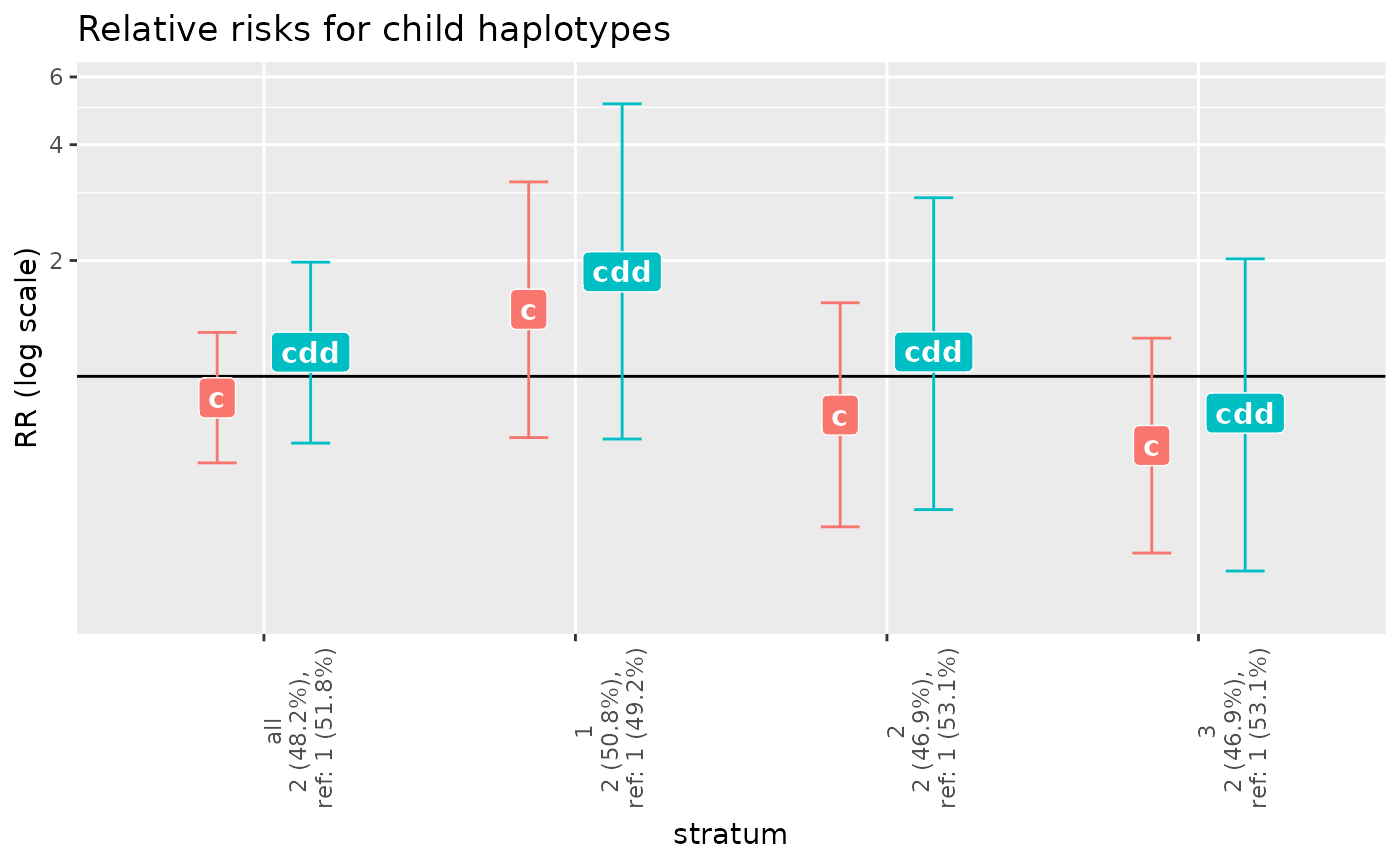
To check the significance of the interaction, we need to use
gxe function
gxe(g_x_me_results)
#>           gxe.test     chisq df      pval
#> 1       haplo.freq 0.5026134  2 0.7777838
#> 2            child 2.9488102  4 0.5664281
#> 3 haplo.freq.trend 0.3731476  1 0.5412935
#> 4      child.trend 2.6559459  2 0.2650139
The p-values here show that the interaction was not significant.
Parent-of-origin-methylation interactions
Similarly, we can also check for interaction between the methylation level and parent-of-origin effect of the genetic marker.
poo_x_me_results <- haplinStrat(
  data = gen_ex_strat_prep,
  strata = 2,
  poo = TRUE
)
#> Warning: Can only (for the time being) use reference = "ref.cat" or
#> "population" when poo == TRUE. Has been changed to "ref.cat".
#>
#> ## Running haplinStrat ##
#>
#> Selected stratification variable: dnam_c.c
#> Frequency distribution of stratification variable:
#>  1  2  3
#> 67 66 67
#>
#> Running Haplin on full data file...Done
#>
#> Running Haplin on stratum "1"...Done
#>
#> Running Haplin on stratum "2"...Done
#>
#> Running Haplin on stratum "3"...Done
haptable(poo_x_me_results)
#>   stratum row.str marker alleles  counts    HWE.pv Original After.rem.NA
#> 1     all       1     m1     1/2 607/593 0.3708224      200          200
#> 2     all       2   <NA>    <NA>    <NA>        NA      200          200
#> 3       1       1     m1     1/2 178/224 0.4912064       67           67
#> 4       1       2   <NA>    <NA>    <NA>        NA       67           67
#> 5       2       1     m1     1/2 206/190 0.6861466       66           66
#> 6       2       2   <NA>    <NA>    <NA>        NA       66           66
#> 7       3       1     m1     1/2 223/179 0.1415450       67           67
#> 8       3       2   <NA>    <NA>    <NA>        NA       67           67
#>   After.rem.Mend.inc. After.rem.unused.haplos pv.overall haplos haplofreq
#> 1                 200                     200  0.4215675      1 0.5176705
#> 2                 200                     200  0.4215675      2 0.4823295
#> 3                  67                      67  0.6427490      1 0.4930795
#> 4                  67                      67  0.6427490      2 0.5069205
#> 5                  66                      66  0.6552084      1 0.5308702
#> 6                  66                      66  0.6552084      2 0.4691298
#> 7                  67                      67  0.4587525      1 0.5302072
#> 8                  67                      67  0.4587525      2 0.4697928
#>   haplofreq.lower haplofreq.upper reference RRcm.est. RRcm.lower RRcm.upper
#> 1       0.4700483       0.5670651       ref 1.0000000  1.0000000   1.000000
#> 2       0.4329349       0.5299517        -  0.9551130  0.6125346   1.512641
#> 3       0.4078670       0.5757597       ref 1.0000000  1.0000000   1.000000
#> 4       0.4242403       0.5921330        -  1.5606351  0.6593474   3.661163
#> 5       0.4479463       0.6150836       ref 1.0000000  1.0000000   1.000000
#> 6       0.3849164       0.5520537        -  0.8267190  0.3738303   1.870074
#> 7       0.4480859       0.6138420       ref 1.0000000  1.0000000   1.000000
#> 8       0.3861580       0.5519141        -  0.7716568  0.3761164   1.625104
#>   RRcm.p.value RRcf.est. RRcf.lower RRcf.upper RRcf.p.value RRcm_RRcf.est.
#> 1           NA 1.0000000  1.0000000   1.000000           NA       1.000000
#> 2    0.8578440 0.7964699  0.4988981   1.294462    0.3508241       1.202628
#> 3           NA 1.0000000  1.0000000   1.000000           NA       1.000000
#> 4    0.3100549 1.4407954  0.6019219   3.440700    0.4240687       1.080438
#> 5           NA 1.0000000  1.0000000   1.000000           NA       1.000000
#> 6    0.6510574 0.7508834  0.3337436   1.712289    0.5004946       1.100715
#> 7           NA 1.0000000  1.0000000   1.000000           NA       1.000000
#> 8    0.4954824 0.5381458  0.2415788   1.232018    0.1409641       1.432857
#>   RRcm_RRcf.lower RRcm_RRcf.upper RRcm_RRcf.p.value RRdd.est. RRdd.lower
#> 1       1.0000000        1.000000                NA 1.0000000  1.0000000
#> 2       0.7367299        1.980414         0.4609985 1.1497242  0.6795373
#> 3       1.0000000        1.000000                NA 1.0000000  1.0000000
#> 4       0.4823310        2.468996         0.8399792 1.8820947  0.6829190
#> 5       1.0000000        1.000000                NA 1.0000000  1.0000000
#> 6       0.4520536        2.759066         0.8271603 1.1445511  0.4635546
#> 7       1.0000000        1.000000                NA 1.0000000  1.0000000
#> 8       0.6120656        3.383351         0.4057060 0.7890665  0.3166753
#>   RRdd.upper RRdd.p.value
#> 1   1.000000           NA
#> 2   2.012892    0.6007082
#> 3   1.000000           NA
#> 4   4.944720    0.2225700
#> 5   1.000000           NA
#> 6   2.997610    0.7579938
#> 7   1.000000           NA
#> 8   2.051910    0.6357477
plot(poo_x_me_results)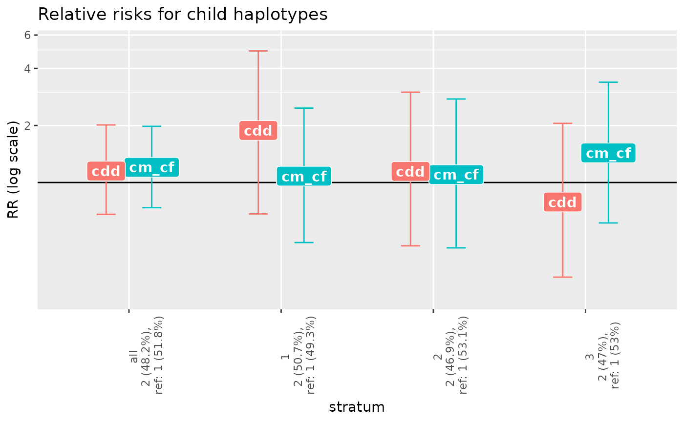
gxe(poo_x_me_results)
#>           gxe.test     chisq df      pval
#> 1       haplo.freq 0.5026134  2 0.7777838
#> 2              poo 0.2626489  2 0.8769332
#> 3 haplo.freq.trend 0.3731476  1 0.5412935
#> 4        poo.trend 0.2175134  1 0.6409412